The most useful and least used in common practice due to lack of knowledge is the VLOOKUP function of MS Excel.
Here I am presenting with the help of one example the common use of VLOOKUP function.
Let us first see the function:
With the VLOOKUP function, ypu can look for specified data in the first column of a table. The result is returned from the column number specified, if found.The formula for VLOOKUP is:
=vlookup(lookup_value,table_array,col_index_num,range_lookup)
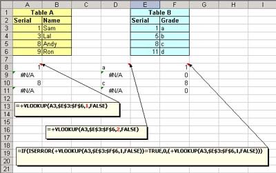
Let us look at the example, I want to see if value in column A3 to A6 of table A exist in Table B.If yes, I want formula to return me column E's value.
The formula is:
=+VLOOKUP(A3,$E$3:$F$6,1,FALSE)
Now, here I am looking for A3(lookup_value) of table A in E3 to F6(table_array), remember: it will look into left most column,so in E3 to E6,and return me value from column 1(col_index_num) which is E3 to E6.Then comes the range_lookup which is False.The Reason for it being False is,the use of False as the optional range_lookup Argument. This directs to the VLOOKUP to find an exact match and is most often needed when looking for a text match. If this is omitted, or True, you will often get unwanted results when searching for text that is in an unsorted column of data. When True is used, or the range_lookup Argument is ignored, the data should be sorted (by the first column) in ascending order.
See the results in column A8 to A11.
Now, if I want to return the value from column F of Table B, all I have to do is to change column index to 2.
=+VLOOKUP(A3,$E$3:$F$6,2,FALSE)
See the results in column D8 to D11.
Whenever, match is not found, the formula will retorn an error i.e. #N/A.To avoid this, i write another formula:
=IF(ISERROR(+VLOOKUP(A3,$E$3:$F$6,1,FALSE))=TRUE,0,(+VLOOKUP(A3,$E$3:$F$6,1,FALSE)))
Meaning that if vlookup returns error i.e. #N/A, then return 0 else return vlookup value.
That is all to it.Hope you find it useful.