Find Cells which have Strikethrough Text or numbers in MS Excel

To Find Cells which have Strikethrough Text or numbers in MS Excel:

• -          Select a cell in the worksheet
• -          Go to the "Find and Select" button and choose "Find"
• -          Click "Options",  and then click the "Format" button”.
• -          Click the "Font" tab.
• -          Select the box Strikethrough" to place a check in it, and then click "OK."
• -          Click "Find All"
• -          A list of every cell that has strikethrough text or number in it will show up
• -          Click on the name of a cell in the list to go to particular cell.

The INDIRECT function in MS Excel

The INDIRECT function is very useful in case you have derived or calculated in a cell the cell reference from where you want the data from.

For Example, if cell A3 has a value C5 (May Be calculated based on some formula or logic) and you want to refer C5 from A3 to get the value of cell C5:

=Indirect(A3)

Remove Leading Spaces in MS Excel

Many times =Trim(Text) and =Trim(Clean(Text)) does not work in MS Excel to remove and clean leading spaces created due to non-breaking space (Char(160)) specially if you are copying data from web or bullet list in MS Word into an Excel Worksheet.

This problem can be resolved by :

=TRIM(CLEAN(SUBSTITUTE(Old Text,CHAR(160)," ")))

Create Bullet in MS Excel

To create the bullet character, press ALT+0149 (Press Alt and type 0149 on the numeric keypad and release Alt).

MS Excel: Get preceding Zero of fixed width text field

When you open csv file in MS Excel, for any text field as number with preceding Zero, excel treats them as number and remove the preceding Zero.

Let us say, that field is 5 characters long:

00542

Excel will open it as (Assume in cell A1):

542

You can use the following formula to get back the Zero:

=Text(A1,”00000”)

See the example below:

MS Excel: Lookup instead of Vlookup or Hlookup

The limitation of vlookup is that you can only lookup in the first column of array and bring back results from it or any column right of it. 

Similar limitation in Hlookup where you can only lookup in first row of array and bring back result from it or any row below it.

To get over with this limitation, use lookup instead of vlookup and Hlookup:

=lookup(Lookup Value, Lookup Vector, Result Vector)

See the examples below:

Use of Lookup for Vlookup

Use of lookup for Hlookup

MS Excel : IfError function in Excel 2010

Iferror is new function in MS Excel 2010 to make life simple. It works as:

= IFERROR(value, value_if_error)

See it's use with vlookup below:

=Iferror(vlookup(A1,Sheet2!A1:C60, 3,False),”Not Found”)

In this formula, if vlookup returns error because value is not found, instead of returning  #N/A, it will return “Not Found”.

MS Excel: Show Alphabetic Row or Column Number

To show row number in alphabetic order, simply right this formula is first location where you wish to start the alphabet i.e. A and then, drag and paste the formula in rows below:

=SUBSTITUTE ((ADDRESS (1, ROW (A1), 4)), 1,"")

Same the case of alphabetical column numbers, at start point, write the following formula and drag and paste on adjacent columns:

=SUBSTITUTE ((ADDRESS (1, Column (A1), 4)), 1,"")

MS Excel: DATEDIF function

The DATEDIF function can be used to calculate the number of days/moths/years between two dates in versions of Excel from 97 to 2007.

=DATEDIF(B9,C9,"m")/12

=DATEDIF(B9,TODAY(),"d")

=DATEDIF(B9,C9,"m")

It is interesting to note that DATEDIF is not listed with other functions under the formula tab in Excel 2007.

Folder and File Option : Missing Security Tab: Windows XP

Problem: Right clicking on folder or file not showing security tab:


Go to Explorer -> tools -> folder options -> View->

navigate to the last check box in the list “USE SIMPLE FILE SHARING” .

Uncheck this checkbox and click OK.

Now you will be able to see the security tab in file properties.

Allow only numeric value in a textbox on a form

Remove //** From the html codes:

This is the function in the header tag

function AllowNumeric(e) {
var iKeyCode = 0;
if (window.event)
iKeyCode = window.event.keyCode
else if (e)
iKeyCode = e.which;
if (iKeyCode > 47 && iKeyCode < 58)
return true
else
return false;

Here is the HTML for the textbox

//////(<)//**
INPUT onkeypress="javascript: return AllowNumeric(event);" id="txtAcctNo" style="WIDTH: 120px; HEIGHT: 20px"
type="text" maxLength="8" runat="server" size="14"
//**>///////

The VLOOKUP Function:Very useful and very simple

The most useful and least used in common practice due to lack of knowledge is the VLOOKUP function of MS Excel.
Here I am presenting with the help of one example the common use of VLOOKUP function.
Let us first see the function:
With the VLOOKUP function, ypu can look for specified data in the first column of a table. The result is returned from the column number specified, if found.The formula for VLOOKUP is:

=vlookup(lookup_value,table_array,col_index_num,range_lookup)



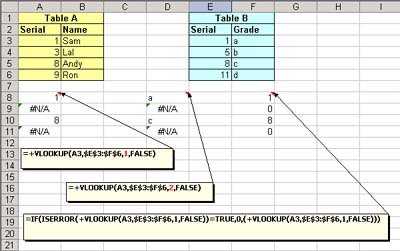
Let us look at the example, I want to see if value in column A3 to A6 of table A exist in Table B.If yes, I want formula to return me column E's value.
The formula is:

=+VLOOKUP(A3,$E$3:$F$6,1,FALSE)

Now, here I am looking for A3(lookup_value) of table A in E3 to F6(table_array), remember: it will look into left most column,so in E3 to E6,and return me value from column 1(col_index_num) which is E3 to E6.Then comes the range_lookup which is False.The Reason for it being False is,the use of False as the optional range_lookup Argument. This directs to the VLOOKUP to find an exact match and is most often needed when looking for a text match. If this is omitted, or True, you will often get unwanted results when searching for text that is in an unsorted column of data. When True is used, or the range_lookup Argument is ignored, the data should be sorted (by the first column) in ascending order.

See the results in column A8 to A11.

Now, if I want to return the value from column F of Table B, all I have to do is to change column index to 2.

=+VLOOKUP(A3,$E$3:$F$6,2,FALSE)

See the results in column D8 to D11.

Whenever, match is not found, the formula will retorn an error i.e. #N/A.To avoid this, i write another formula:

=IF(ISERROR(+VLOOKUP(A3,$E$3:$F$6,1,FALSE))=TRUE,0,(+VLOOKUP(A3,$E$3:$F$6,1,FALSE)))

Meaning that if vlookup returns error i.e. #N/A, then return 0 else return vlookup value.
That is all to it.Hope you find it useful.

Export Custom Outlook Form Data to MS Access

Dim appAccess
Dim nms
Dim strFolder
Dim fld
Dim strAccessPath
Dim rst
Dim dbe
Dim wks
Dim dbs
Dim itms
Dim itm

Sub CommandButton1_Click()

Set nms = Application.GetNamespace("MAPI")
strFolder = "fbtest folder"
Set fld = nms.Folders("Personal Folders").Folders(strFolder)

'Pick up path to Access database directory from Access SysCmd function
Set appAccess = CreateObject("Access.Application")
strAccessPath = appAccess.SysCmd(9)

'Get DAO version from DBEngine
strDBEngine = appAccess.Application.DBEngine.Version

'MsgBox "DBEngine version: " & strDBEngine

appAccess.Quit

If strDBEngine = "3.51" Then
'Office 97 DAO version
Set dbe = CreateObject("DAO.DBEngine.35")
strDBName = strAccessPath & "fbtestdb.mdb"
ElseIf strDBEngine = "3.6" Then
'Office 2000 DAO version
Set dbe = CreateObject("DAO.DBEngine.36")
strDBName = strAccessPath & "fbtestdb.mdb"

Else

MsgBox "Unknown Office version; canceling"

Exit Sub

End If
'MsgBox "DBName: " & strDBName
Set wks = dbe.Workspaces(0)
Set dbs = wks.OpenDatabase("S:\sameer\fbtestdb.mdb")

'Open Access table containing contact data
Set rst = dbs.OpenRecordset("fbtesttable")
'Set up reference to Outlook folder of items to export

Set itms = fld.Items
ItemCount = itms.Count
If ItemCount = 0 Then
MsgBox "No FB requests to export"

Exit Sub
Else

MsgBox ItemCount & " FB requests to export"

End If
'Set up reference to Outlook folder of items to export
Set itms = fld.Items
ItemCount = itms.Count

If ItemCount = 0 Then

MsgBox "No Fund Builder requests to export"

Exit Sub
Else

MsgBox ItemCount & " FB requests to export"

End If
For Each itm In itms

rst.AddNew

'Custom Outlook properties
rst.Request=itm.userproperties("001 Request")
rst.AccountNumber=itm.userproperties("002 Account Number") rst.ClientName=itm.userproperties("002 Client Name")

rst.Update

Next

rst.Close

MsgBox "All FB requests exported!"

End Sub

Export Data From Outlook Custom Form to Excel

Sub CommandButton1_Click()
ExportToExcel()
End Sub

Sub ExportToExcel()

Dim appExcel
Dim olMAPI
Dim strTemplatePath
Dim strSheet
Dim Ifld
Dim MItem

Set olMAPI = GetObject("", "Outlook.Application").GetNameSpace("MAPI")
Set Ifld = olMAPI.Folders("Personal Folders").Folders("SamTest")

i=1

'Pick up Template path from the word options dialog
strTemplatePath="H:\"

'Debug.Print "Document folder: " & strTemplatePath

strSheet="SameerTest.xls"
strSheet=strTemplatePath & strSheet

'Set appExcel= New Excel.Application
Set appExcel=GetObject("", "Excel.Application")

appExcel.Workbooks.Open (strSheet)
Set wkb = appExcel.ActiveWorkBook
Set wks =wkb.Sheets(1)
wks.Activate
wks.Cells(1, 1)="Subject"
wks.Cells(1,2)="ClientName"
wks.Cells(1,3)="ClientAddress"
wks.Cells(1,4)="ClientAge"

appExcel.Application.Visible=TrueFor Each MItem In Ifld.Items

If Left(MItem.Subject, 12) = "Client Form" Then
i = i + 1

If MItem.Subject<>"" Then
wks.Cells(i,1).Value = MItem.Subject
End If

If MItem.UserProperties("010 ClientName").Value<>"" Then
wks.Cells(i,2).Value = MItem.UserProperties("010 ClientName").Value
End If

If MItem.UserProperties("020 ClientFirstName").Value<>"" Then
wks.Cells(i,3).Value = MItem.UserProperties("020 ClientAddress").Value
End If

If MItem.UserProperties("030 ClientInitial").Value<>"" Then
wks.Cells(i,4).Value = MItem.UserProperties("030 ClientAge").Value
End If End If

Next

Set MItem = Nothing
Set Ifld = Nothing
Set strTemplatePath = Nothing
Set strSheet = Nothing
Set olMAPI = Nothing
Set appExcel = Nothing

End Sub

Counting Commas or Special characters in a cell

Suppose, your names seperated by "," is in cell A4.

Here is the formula to calculate number of commas in the cell A4:

=LEN(A4)-LEN(SUBSTITUTE(A4,",",""))


The first part: LEN(A4) calculates length of string with commas.

The Second part: LEN(SUBSTITUTE(A4,",","")) calculates length of string without commas.

The differnece of the two i.e. first part-second part will give you number of commas in your string.

This formula can come out handy in many calculations.

VB 6.0-Some Formatting Expression

I find it very handy:

Formatting numbers with named formats Expression Result
Format(35988.3708, "general number") 35988.3708
Format(35988.3708, "currency") $35,988.37
Format(-35988.3708, "currency") ($35,988.37)
Format(35988.3708, "fixed") 35988.37
Format(1, "fixed") 1.00
Format(35988.3708, "standard") 35,988.37
Format(1, "standard") 1.00
Format(0.35988, "percent") 35.99%
Format(0, "Yes/No") No
Format(0.35988, "Yes/No") Yes
Format(0, "True/False") False
Format(342, "True/False") True
Format(0, "On/Off") Off
Format(-1, "On/Off") On


Formatting numbers with special characters Expression Result
Format(35988.3708, "00000.0") 35988.4
Format(35988.3708, "0000000.0") 0035988.4
Format(35988.3708, "00,000.00000") 35,988.37080)
Format(6.07, "0.###") 6.07
Format(6.07, "0.000##") 6.070
Format(143879, "#,###,###.00") 143,879.00

Formatting numbers with embedded characters Expression Result
Format(45, "\[00\]") [45]
Format(642, "\£000.00") £642.00
Format(99, "00\¢") 99¢
Format(8, "#0\).") 8).

Formatting dates and time

Format(36715.5784, "general date") 7/8/00 1:52:54 PM
Format(36715.5784, "short date") 7/8/00
Format(36715.5784, "medium date") 08-Jul-00
Format(36715.5784, "long date") Saturday, July 08, 2000
Format(36715.5784, "short time") 13:52
Format(36715.5784, "medium time") 01:52 PM
Format(36715.5784, "long time") 1:52:54 PM
Format(36715.5784, "c") 7/8/00 1:52:54 PM
Format(36715.5784, "d") 8
Format(36715.5784, "dd") 08
Format(36715.5784, "ddd") Sat
Format(36715.5784, "dddd") Saturday
Format(36715.5784, "ddddd") 7/8/00
Format(36715.5784, "dddddd") Saturday, July 08, 2000
Format(36715.5784, "w") 7
Format(36715.5784, "ww") 28
Format(36715.5784, "m") 7
Format(36715.5784, "mm") 07
Format(36715.5784, "mmm") Jul
Format(36715.5784, "mmmm") July
Format(36715.5784, "q") 3
Format(36715.5784, "y") 190
Format(36715.5784, "yy") 00
Format(36715.5784, "yyyy") 2000
Format(36715.5784, "h") 13
Format(36715.5784, "hh") 13
Format(36715.5784, "n") 52
Format(36715.5784, "nn") 52
Format(36715.5784, "s") 54
Format(36715.5784, "ss") 54
Format(36715.5784, "ttttt") 1:52:54 PM
Format(36715.5784, "AM/PM") PM
Format(36715.5784, "am/pm") pm
Format(36715.5784, "A/P") P
Format(36715.5784, "a/p") p
Format(36715.5784, "AMPM") PM

Format "w" returns day of week (1 = Sunday, 7 = Saturday)
Format "ww" returns week of year (1-53)
Format "y" returns day of year (1-366)
Format "h" returns hour of day as one or two digits...if necessary
Format "hh" returns hour of day as two digits...definitely
Above applies to "n"/"nn", and "s"/"ss" as well
Format "AMPM" uses settings from WIN.INI [intl] s1159=AM, s2359=PM
Try mixing and matching the format strings Expression Result
Format(36715.5784, "m-d-yy") 7-8-00
Format(36715.5784, "d-mmmm-y") 8-July-00
Format(36715.5784, "mmmm yyyy") July 2000
Format(36715.5784, "hh:mm a/p") 01:52 p
Format(36715.5784, "m/d/yy h:mm") 7/8/00 13:52

FormatDateTime
This new function works about the same as the regular Format function, but you're only allowed to
use one of 5 constants -
vbGeneralDate, vbLongDate, vbShortDate, vbLongTime, vbShortTime.

MS Excel: Working in multi-sheet environment

When we are referencing one sheet data to another sheet in a formula or otherwise comparing multi sheets in a work book, it becomes tedious to move from sheet to sheet back and forth. Think of a situation where you have to refer data from three or four sheet.

Wouldn't it be nice, if you can have all those three sheets of workbook open side by side?
Did you know that there is an easy way to do this and I always find it very handy while working on a multi-sheet workbook?

Open your workbook, sheet1.

Go to Window tab,
Click on New Window,
Select sheet 2 on this newly opened workbook where you will see on the top with the name: 2.




Again repeat the same steps and open sheet 3. Here with the name, you will see: 3.

Now, that you have the same workbook opened thrice with different sheets,

Go to window,
Click arrange,
Select Vertical

and here you go, three sheet of same workbook opened side by side, toggle around and enjoy working on multi-sheet workbook.

MS Excel: Close all Open Workbooks

At times, when you have many workbook open on your desktop and wish to close all of them together,there is an easy way in MS Excel to do this. I could never understand the reason why this option is not on main menu and is kept hidden.
Follow this:

Press Shift key on the keyboard while clicking File on the menu;

And now you will see the option: Close All

Click on it and all the workbooks are closed unless, in some workbook(s), you have made changes and not saved them.Excel will prompt you to save changes and close the workbooks.

MS Excel: Not only sort data in a column but also in the rows

Click a cell of the row you want to sort horizontally.

Select Sort from the Data menu.

In the Sort dialog box, click on the Options.

In the Sort Options dialog box, click on Sort Left to Right, then click OK.

Back in the Sort dialog box, go to the Sort By combo box and select a row to sort, and also select the direction (ascending or descending).

You can select additional rows by going to the boxes.

Click OK.
Yu Hooo!!! Excel sorts the row horizontally.

MS Excel: Get Summary Calculations on the Fly

As a busy executive, you are presented with lots of data in MS Excel format. Though you know the formulas to calculate and find results, but it is just a waste of time to write formula to see what the sum of particular range is or which is the highest value or lowest value or may be the average.
While looking at the spreadsheet, you can do the following to improve your analysis capabilities or effectively respond to one off questions which keeps coming up during meetings:


1. From the menu option, select View, and check the status bar.





2. This action will start showing you status bar at the bottom of spreadsheet.

3. Select the range of data you wish to analyze, and you will see on the status bar, Sum= 100 or whatever is the sum of the range selected (By default, excel is set to show Sum).

4. Right click on status bar, and you will see options like Average, Count, Count Nums, Max, Min and Sum. Select any one and see the result on status bar.